Examples for using the one point kite model

Create a test project

mkdir test
cd test
julia --project="."

With the last command, we told Julia to create a new project in the current directory.

Then we add the three required packages to our new project. By pressing the key "]" we enter the package manager mode where we can add or delete packages.

]
add KiteUtils
add KitePodModels
add KiteModels
st
<BACKSPACE>

The command "st" was not really required, but it is useful to display which versions of the packages we have in our project. Another important package manager command is the command "up", which updates all packages to the latest compatible versions.

Then, copy the default configuration files and examples to your new project:

using KiteModels
copy_settings()
copy_examples()

The first command copies the files settings.yaml and system.yaml to the folder data. They can be customized later. The second command creates an examples folder with some examples.

Plotting the initial state

First, an instance of the model of the kite control unit (KCU) is created which is needed by the Kite Power System model KPS3. Then we create a kps instance, passing the kcu model as parameter. We need to declare these variables as const to achieve a decent performance.

using KiteModels
const kcu = KCU(se())
const kps = KPS3(kcu)

Then we call the function find_steady_state which uses a non-linear solver to find the solution for a given elevation angle, reel-out speed and wind speed.

find_steady_state!(kps, prn=true)

To plot the result in 2D we extract the vectors of the x and z coordinates of the tether particles with a for loop:

x = Float64[] 
z = Float64[]
for i in 1:length(kps.pos)
     push!(x, kps.pos[i][1])
     push!(z, kps.pos[i][3])
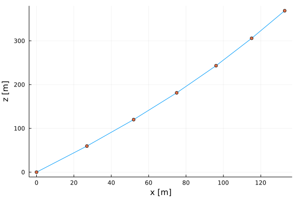
end

And finally, we plot the position of the particles in the x-z plane. When you type using Plots you will be asked if you want to install the Plots package. Just press \<ENTER\> and it gets installed.

using Plots
plot(x,z, xlabel="x [m]", ylabel="z [m]", legend=false)
plot!(x, z, seriestype = :scatter)

Inital State

Print other model outputs

Print the vector of the positions of the particles:

julia> kps.pos
7-element StaticArrays.SVector{7, StaticArrays.MVector{3, Float64}} with indices SOneTo(7):
 [0.0, 0.0, 0.0]
 [26.95751778658999, 0.0, 59.59749511924355]
 [51.97088814144287, 0.0, 120.03746888266994]
 [75.01423773175357, 0.0, 181.25637381120865]
 [96.06809940556136, 0.0, 243.18841293054678]
 [115.11959241520753, 0.0, 305.7661763854397]
 [132.79571663189674, 0.0, 368.74701279158705]

Print the unstretched and stretched tether length and the height of the kite:

julia> unstretched_length(kps)
150.0

julia> tether_length(kps)
150.1461801769623

julia> calc_height(kps)
142.78102261557189

Print the force at the winch (groundstation, in Newton) and at each tether segment:

julia> winch_force(kps)
592.5649922210812

julia> spring_forces(kps)
6-element Vector{Float64}:
 592.5534481632459
 595.0953689567787
 597.6497034999358
 600.215921248686
 602.793488771366
 605.3855398009119

The force increases when going upwards because the kite not only experiences the winch force but in addition the weight of the tether.

Print the lift and drag forces of the kite (in Newton) and the lift-over-drag ratio:

julia> lift, drag = lift_drag(kps)
(730.5877517655691, 157.36420900755007)

julia> lift_over_drag(kps)
4.64265512706588

Print the wind speed vector at the kite:

julia> v_wind_kite(kps)
3-element StaticArrays.MVector{3, Float64} with indices SOneTo(3):
 12.54966091924401
  0.0
  0.0

Example of reeling out the tether

include("examples/reel_out_1p.jl")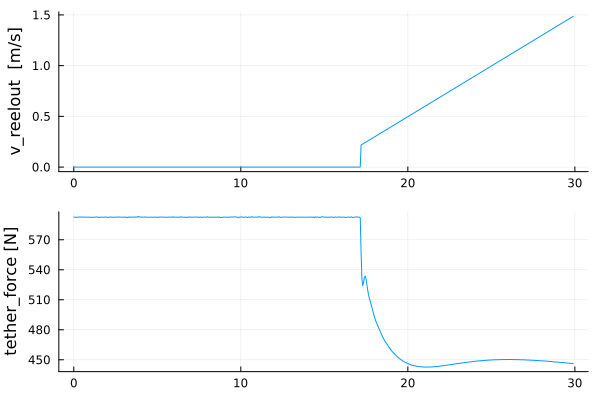

In this example, we first keep the tether length constant and at 15 s start to reel out the winch with an acceleration of 0.1 m/s². At a set speed below 2.2 m/s the brake of the winch is active, therefore the "jump" in the v_reelout at the beginning of the reel-out phase.

It is not a real jump, but a high acceleration compared to the acceleration afterward.