Exporting formatted datasets
Introduction
For analysing CAN bus log files I am exporting the data sets with CAN messages to .csv and then import them in LibreOffice spread sheets. Finally I create Excel files that I can give to my collegues.
The CAN bus is used in cars, wind turbines, electric chargers, UAVs and many other industrial devices for the communication between intelligent sensors, actuators, controllers and user interface devices.
One log file can easily contain millions of messages, therefore Julia is a good choice for statistics, error analysis and graphical presentation of relevant aspects of the CAN bus traffic due to the simplicity, power and performance Julia provides.
But CAN messages are usually hex encoded. So how can we export a dataset with some hex encoded columns?
Creating a test project
For trying out a new package and/or example it is always good to create a new project first. For example using the following commands:
mkdir can
cd can
julia --project="."
And then install the required packages:
julia> using pkg
julia> pkg"add InMemoryDatasets"
julia> pkg"add DLMReader"
julia> pkg"add Printf"
Now quit julia with
julia --project -t auto
This uses the set of packages we just installed and starts julia using all available threads. This is useful when handling large data sets (millions of messages).
Creating a sample data set
using InMemoryDatasets, DLMReader, Printf

ds = Dataset(time=0.0, d1=10, d2=20)
time = 0.1
for i in 1:9
    global time
    ds2 = Dataset(time=time, d1=10+1, d2=20+i)
    append!(ds, ds2)
    time += 0.1
end
ds.d1[4] = missing
If you run this code the dataset should look like this:
julia> ds
10×3 Dataset
 Row │ time      d1        d2
     │ identity  identity  identity
     │ Float64?  Int64?    Int64?
─────┼──────────────────────────────
   1 │      0.0        10        20
   2 │      0.1        11        21
   3 │      0.2        12        22
   4 │      0.3        13        23
   5 │      0.4   missing        24
   6 │      0.5        15        25
   7 │      0.6        16        26
   8 │      0.7        17        27
   9 │      0.8        18        28
  10 │      0.9        19        29
Formatting the output
For formatting the columns d1 and d2 in hex we need the following lines of code:
function round6(value)
    @sprintf("%12.6f", value)
end

function hex(n)
    if ismissing(n) return "--" end
    string(n, base=16, pad=2)
end

setformat!(ds, :time => round6)
setformat!(ds, :d1 => hex)
setformat!(ds, :d2 => hex)
Because our dataset can contain missing values we need to handle the special case
that n is missing. The round6 function is not strictly required, but for easy readability
of the csv output I wanted to have a fixed number of digits for the time stamp.
If we now print the dataset in the REPL we get:
julia> show(ds, show_row_number=false, eltypes=false)
10×3 Dataset
 time          d1  d2
──────────────────────
     0.000000  0a  14
     0.100000  0b  15
     0.200000  0c  16
     0.300000  0d  17
     0.400000  --  18
     0.500000  0f  19
     0.600000  10  1a
     0.700000  11  1b
     0.800000  12  1c
     0.900000  13  1d
Now all columns are nicely formatted. I am using here the keyword parameters show_row_number=false
andeltypes=false to suppress the output of the column types and the row numbers.
Saving this as .csv file is now easy:
filewriter("output.csv", ds, mapformats=true)
The trick is to use the named parameter mapformat=true, if you do that the formatting function
is applied on the .csv output. The resulting file looks like this:
shell> cat output.csv
time,d1,d2
    0.000000,0a,14
    0.100000,0b,15
    0.200000,0c,16
    0.300000,0d,17
    0.400000,--,18
    0.500000,0f,19
    0.600000,10,1a
    0.700000,11,1b
    0.800000,12,1c
    0.900000,13,1d
Importing this with LibreOffice
You can just double click on the file output.csv and a dialog box will open. Just make sure to select the column type text for colum d1 and d2.
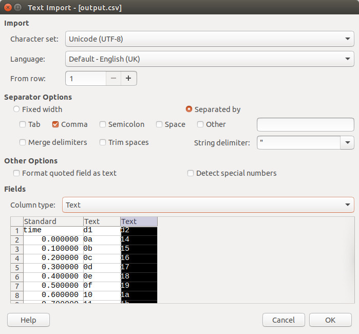
When you click on OK you have a well formatted table which you can save as .odf spreadsheet or in Excel format for further analysis and distribution.