Why am I using Julia?
Introduction
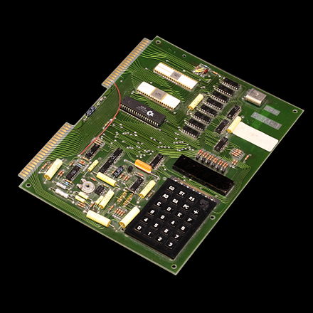
I started programming in 1976 using the KIM 1 and the 6502 machine language. Since then I learned and used many languages, Assembler, Pascal, Delphi, Basic, Foxpro, Java, C, C++, Bash, Matlab, Python and more…
 |
|---|
| KIM 1 |
Why do I think that Julia is superior to all of them in many (not all) applications?
What is so great about Julia?
Reason no. one: speed
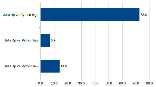
When you need to process large amounts of data speed is important. Julia is a just-in-time compiled language using the mature LLVM compiler infrastructure, so you get fast machine code for different processors. In contrast to Python also multi-threading is well supported. I wrote a simulation package in Python+Numba, and re-wrote it in Julia.
 |
|---|
| Performance advantage of Julia vs Python+Numba |
Depending on the test case Julia was 7 to 70 times faster than Python+Numba. And writing the Julia code was much easier because mixing Python with Numba is a real pain because they look similar, but behave very differently.
If you only use Python with algorithms for which C++ or Fortran libraries are available, then you will not see much of an advantage from using Julia. But if you write new programs or libraries using new algorithms Julia is much faster (if you follow the Performance Tips).
Reason no. two: simplicity and elegance
You can operate with vectors as you would do it in mathematical notation, you can use × for the cross product and ⋅ for the dot product. And functions can return tuples (multiple values), which is very useful.
# pos:        vector of tether particle positions
# v_apparent: apparent wind speed vector
function kite_ref_frame(pos, v_apparent)
    c = pos[end-1] - pos[end]
    z = normalize(c)
    y = normalize(v_apparent × c)
    x = normalize(y × c)
    x, y, z
end
And you can use Greek letters in the code:
using Distributions, Random

T = [84.5, 83.6, 83.6] # temperature measurements
μ = mean(T)            # average cpu temperature
σ = 2.5                # 95.45 % of the measurements are within ± 5 deg
d = Normal(μ, σ)
good = cdf(d, 88.0)    # this percentage of the cpus will not start to throttle
And you can write arrays cleanly:
julia> A = [1 2π
            3 4π]
2×2 Matrix{Float64}:
 1.0   6.28319
 3.0  12.5664
And any scalar function incl. user-defined functions can be applied on a vector using the dot syntax:
julia> sin.([1,2,3])
3-element Vector{Float64}:
 0.8414709848078965
 0.9092974268256817
 0.1411200080598672
Reason no. three: Great REPL (Read, Evaluate and Print Loop)
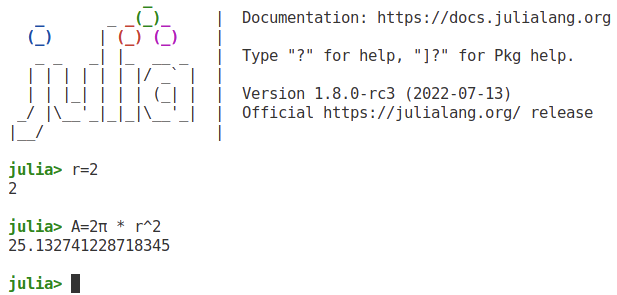
Normally, compiled languages don’t have any REPL, but if you ever used it you do not want to miss it again:
 |
|---|
| Julia REPL |
You can do basic calculations, but also try out any function you want to use. You get help by typing ? and press <Enter>, or help for a specific function by typing for example:
?sin
You can run your scripts using the include function, for example:
include("hello_world.jl")
It has four modes of operation, the julia mode for executing julia code, the help modus, the shell modus (which you reach by pressing ;) and the package manager mode explained in the next section. I always develop code in the REPL and when a line of code (or a function) works I copy it into the script. If you wonder how to get the character π: just type \pi and then the TAB key.
Reason no. four: Built-in package manager
In Python it can be very difficult to install packages. There is pip that might work, but not good for binary dependencies. There is easy_install, there is conda… Many package managers, but all of them only work sometimes, for some packages on some operating systems… On Julia is only one package manager and it works fine with all packages on all supported operating systems (Windows, Mac, Linux…) on ARM and X86.
You can reach the prompt of the package manager by typing ]. It looks like this:
(@v1.8) pkg> st
Status `~/.julia/environments/v1.8/Project.toml`
  [e1d33f9a] DLMReader v0.4.5
  [31c24e10] Distributions v0.25.66
  [5c01b14b] InMemoryDatasets v0.7.7
⌃ [14b8a8f1] PkgTemplates v0.7.26
⌃ [91a5bcdd] Plots v1.29.0
  [0c614874] TerminalPager v0.3.1
Info Packages marked with ⌃ have new versions available
The prompt tells you which environment is active, and you can add, update and delete packages, but also display statistics or download the source code of a package for development. Each Julia package has a clear definition of the versions of the dependencies it works within a file called Project.toml.
Therefore it is easy to write code that will never break in the future. From my point of view thats a killer feature. If required, the package manager also installs pre-compiled C++ or Fortran libraries which works very well.
If you are looking for a specific package, JuliaHub will help you to find it.
Reason no. five: the composability of packages
Julia packages that are written independently often (not always) work together surprisingly well. Example: We have designed a control system, but now we want to do a Monte Carlo analysis to find out how robust it is in the presence of parameter uncertainties.
using ControlSystems, MonteCarloMeasurements, Plots

ω = 1 ± 0.1  # create an uncertain Gaussian parameter
ζ = 0.3..0.4 # create an uncertain uniform parameter

G = tf(ω^2, [1, 2ζ*ω, ω^2]) # systems accept uncertain parameters
Output:
TransferFunction{Continuous, ControlSystems.SisoRational{Particles{Float64, 2000}}}
            1.01 ± 0.2
----------------------------------
1.0s^2 + 0.7 ± 0.092s + 1.01 ± 0.2

Continuous-time transfer function model
The function tf which was originally written for real parameters only, when supplied with uncertain parameters it calculates and prints the correct result. Magic! 😄
Now lets plot the result for the frequency range 0.01 to 100 rad/s on a logarithmic scale:
w = exp10.(-2:0.02:2)
bodeplot(G, w)
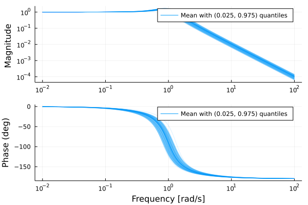
Plotting of diagrams with uncertainty works, even though the packages Plot.jl and MonteCarloMeasurements.jl were developed independently by different authors. You can also combine calculations with physical units and get plots that show the correct physical units. Just magic! 😄
This is so much better than Python or C++ where every library comes with its own implementation of types like vectors that are not compatible with each other. In Julia, you write a generic library, and then it can work with StaticArrays.jl (stack allocated) or normal arrays (heap allocated) or sparse arrays or whatever and it just works.
Reason no. six: an awesome community
If you ask a question on discourse you usually get an answer within 15 minutes. And half of the people that reply are scientists, they know what they are talking about. So you get very qualified answers quickly, often some extra information that might help you to improve your approach.
State-of-the-art solvers for differential equations
If you are creating models of physical, chemical or biological systems, you will often need to solve differential equations. The package DifferentialEquations.jl provides the world’s best set of solvers for these kind of problems.
State-of-the-art optimizers
If you want to optimize a system for example minimize the costs or the time or other properties of a system you need a mathematical optimizer. JuMP provides a domain-specific modeling language for mathematical optimization embedded in Julia. This is easy to use, fast and powerful. For example here is a solution of the Rosenbrock function:
using JuMP
import Ipopt

model = Model(Ipopt.Optimizer)

@variable(model, x)
@variable(model, y)
@NLobjective(model, Min, (1 - x)^2 + 100 * (y - x^2)^2)

optimize!(model)

println("x: ", value(x))
println("y: ", value(y))
The Scientific Machine Learning ecosystem
The SciML ecosystem provides a unified interface to libraries for scientific computing and machine learning. So far I mainly used NonlinearSolve and Optimization.jl for root-finding and for optimization problems where JuMP is not the best choice. The unified interfaces make it easy to try different solvers to find the best one for your problem.
If you are modeling real-world problems like the Corona disease then combining differential equations and machine learning can give superior results.
Limitations
Limitations of language/ compiler and tooling
Compilation and load times
Loading packages takes some time, and also the just-in-time compilation kicks in when you make your first function call. This is known as the time-to-first-plot problem (TTFP). Simple example:
using Plots
p = plot(rand(2,2))
display(p)
If we now save this code in the file ttfp.jl run the program with the command:
@time include("ttfp.jl")
we will see that it takes about 9 seconds on a computer with an i7-7700K CPU. This is quite a lot of time for such a small program. There a different approaches to mitigate this issue. What I usually do is create a system image with all packages I use for a curtain project and do an ahead-of-time compilation of these packages. I will explain in a separate blog post how to do that. If you are curious already, have a look at PackageCompiler.jl.
There is an ongoing effort to use binary caches of the compiled code so that you need to recompile only when the source code has changed, but it will take some time until this will work without any user interaction.
UPDATE 2024: With Julia 1.10.0 this time is down to about 2s. So PackageCompiler is now only needed if you use very large packages like ModelingToolkit.jl.
For use on embedded systems
Currently, with Julia 1.8 the first issue is the amount of RAM that is needed: Using Julia with less than 4GB RAM is not very enjoyable. A cross-compiler is missing. For these reasons writing code for smaller embedded systems is not feasible. The smallest system I would use with Julia is a Raspberry Pi 4 and a 64-bit OS.
I know that the Julia developers work hard to mitigate these issues, so in a few years, Julia will hopefully also be usable for smaller embedded systems.
Working with modules
While working with modules is supported by the language, using modules that are NOT packages is not well supported by the tooling. The VSCode Julia plugin will NOT find symbols of modules in the LOAD_PATH, see this bug report. Workarounds exist, but I find them ugly. As a consequence I use only one module per app/ package and split the program using includes. This is not so good because a file is no longer a stand-alone unit of code that you can read on its own and requires some adaptation of your habits if you are an experienced C++ or Python programmer.
Limitations of the ecosystem
- There is no easy-to-use, well-integrated GUI library. Yes, you can use QML.jl or GTK4.jl and many others, but they all have their issues, one of the issues is the lack of Julia specific documentation.
Luckily you can use most Python and R libraries from within Julia, so the lack of a specific library is usually no show-stopper. Have a look at PythonCall.jl and RCall.jl. Also Fortran and C code can be called directly from Julia, for C++ you need an interface library like CxxWrap.
Conclusions
If you want to analyze data, model physical systems, design control systems or create a web portal with dynamic data Julia is a good choice for you. Also if you do number crunching on graphic cards or clusters. So far it is not a good choice for mobile apps or small embedded systems. It can also be used for machine learning, but I am not qualified to say how well that works (I guess it depends…)
So give Julia a try if you are now using Python, Matlab, Fortran or C++ for one of the mentioned tasks. Your life will become happier…
Acknowledgments
Thanks to Fredrik Bagge Carlson for providing the example for composability .